

Databricks spend grows for two different reasons, and the right fix depends on which one is actually happening. Data observability tools for Databricks show where the money and the failures are coming from, down to the job, the cluster and the team, and then leave a person, or an automation that person configures, to act on what they find. Execution engines work further down the stack: they change how fast the same Spark code runs, which cuts compute-hours directly without anyone touching a notebook. Most teams need both, applied in order: visibility first, to find out where the hours concentrate, and a faster engine wherever the remaining cost turns out to be pure CPU time.
The two layers get bought, built and operated separately, which is why data observability tools for Databricks and execution engines get confused so often. One watches a system that already runs: Databricks’ own system tables, cluster metrics, query logs, job run history. A second category changes what sits underneath those same jobs, translating the identical Spark plan into different CPU instructions. Mixing them up leads a team to expect a dashboard to lower next month’s bill by itself, or to expect a faster runtime to explain where last month’s spend actually went. Neither does the other’s job.
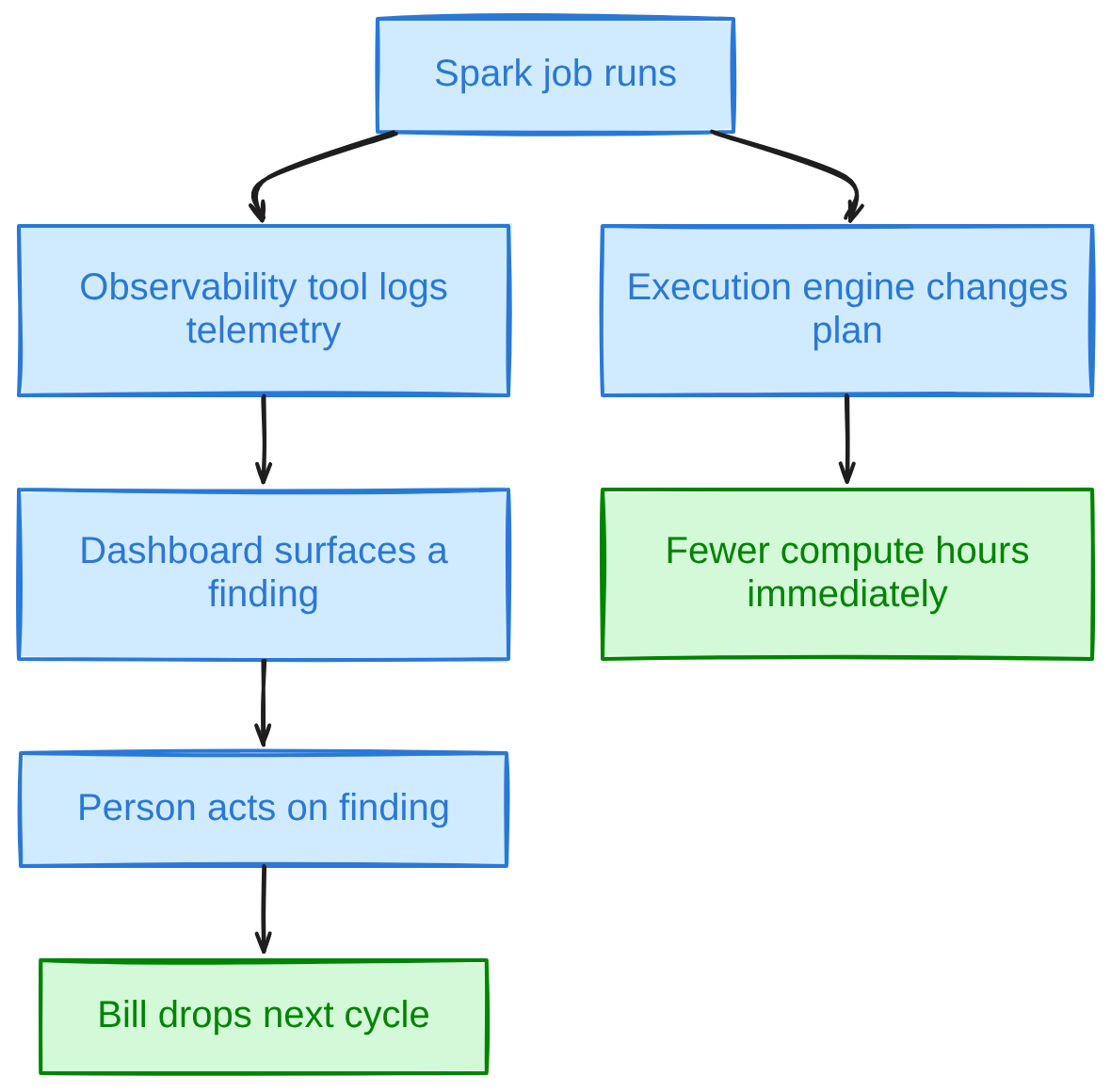
This guide covers what each layer does, what Databricks ships natively, where observability earns its keep, where a different execution engine pays for itself, and how to sequence the two instead of picking a side. It closes with a short look at where observability and execution products differ on pricing, lock-in and the kind of problem each one actually solves.
Observability Tools and Execution Engines: What Each One Is
Observability tools and execution engines sit at different layers of a Databricks estate: one watches spend and failures after they happen, the other changes how a job’s compute gets produced in the first place.
What Are Data Observability Tools for Databricks?
Under the cost and performance banner, data observability tools for Databricks collect telemetry from system tables, cluster metrics and job run history and turn it into attribution: which job, cluster or team produced a given dollar of spend or a given failure. Representative categories include native platform telemetry, dedicated cost and performance observability products such as Unravel Data, and data-quality observability products such as Monte Carlo, Bigeye or Metaplane, which watch freshness, volume, schema and lineage rather than compute-hours. None of them change what a job executes. They change what a team can see about it.
What Is an Execution Engine for Databricks?
An execution engine is the layer that turns a parsed, optimized query plan into actual CPU work: standard JVM Spark, Databricks’ own Photon, or an open-source native engine such as Apache Gluten or DataFusion Comet plugged into the same Spark job. Swapping or tuning the engine changes how many compute-hours a job burns to produce a given result. It does not say which job is burning them in the first place, which is the complementary half of the picture observability covers.
| Feature | Observability Tools | Execution Engines |
|---|---|---|
| Primary function | Attribute spend and failures to a job, cluster or team | Turn the same query plan into CPU work, faster |
| Changes the Spark code? | No | Sometimes none, depending on the engine and its operator coverage |
| Changes the bill directly? | No, a person has to act on the finding first | Yes, fewer compute-hours shows up on the next invoice |
| Typical output | Dashboard, alert, attribution report, tuning recommendation | Lower wall-clock time and compute-hours on the jobs it runs |
| Example categories | Native system tables, Spark UI, Unravel Data, data-quality monitors | Photon, Apache Gluten with Velox, DataFusion Comet |
Two Kinds of Observability: Data Quality vs Cost and Performance
Observability for a Databricks estate actually covers two distinct jobs, and which one a team means depends on what is failing: the data itself or the compute that produced it. Data observability watches the tables: freshness windows, volume and row-count drift, schema changes, null spikes, and lineage from source to BI dashboard, the domain of products such as Monte Carlo, Bigeye and Metaplane. Cost and performance observability, the other half and the one most data observability tools for Databricks buying decisions actually target, watches the compute that produced those tables instead: job and cluster telemetry, DBU attribution by tag, and query-level diagnostics, largely the domain of system tables, Spark UI, query profile and dedicated products such as Unravel Data.
A table can be fresh and correctly shaped while the cluster that built it ran three times longer than it needed to.
What Databricks Gives You Natively
Databricks ships a working slice of cost observability before anyone buys anything extra: system tables for billing and compute, a query profiler, budgets, tags and compute policies that between them cover a meaningful share of the job natively.
system.billing.usage records hourly-granularity, account-wide billable usage, with columns for sku_name, usage_quantity, usage_unit, custom_tags, usage_metadata and identity_metadata. Records typically land within about 12 hours of actual usage, longer for brand-new workspaces, and Databricks appends two new records rather than mutating history whenever a billing correction occurs, which matters for anyone comparing a before-and-after number too soon after a billing period closes.
Alongside it, system.billing.list_prices gives list pricing for reference, and system.compute.node_timeline provides minute-by-minute utilization for all-purpose, jobs and Lakeflow pipeline compute: the same raw material that data observability tools for Databricks or a hand-written query draw on to find an idle cluster. Notably, node_timeline does not cover serverless compute or SQL warehouses, a real gap in the native picture, and nodes running under 10 minutes may not appear in it at all.
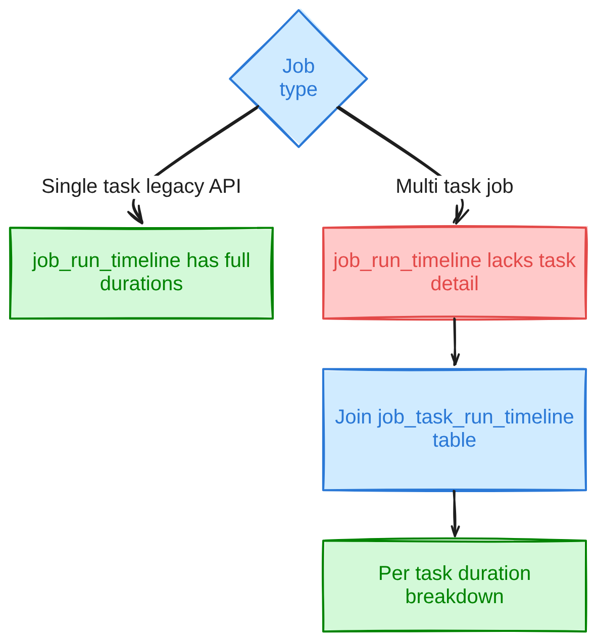
system.lakeflow.job_run_timeline tracks job runs account-wide across every workspace in the same cloud region, with 365 days of free retention, and system.query.history adds query-level detail for SQL work. Granular duration columns, setup, queue, run, cleanup and execution, populate directly on job_run_timeline only for single-task jobs built on the legacy Jobs API; multi-task jobs get the equivalent per-task breakdown from the separate system.lakeflow.job_task_run_timeline table instead, which means diagnosing a slow multi-task pipeline natively means joining two tables rather than reading one.
Query Profile visualizes per-task time, rows processed and memory for a single SQL query to find its slowest stage, and surfaces automated performance insights pointing at specific tuning opportunities; the Spark UI covers the fuller, multi-stage application view that a complex job needs. Both are native and free. Both still need a person to open them, read them and act, which is the limit every native tool shares: detection without automatic remediation.
Databricks Budgets track spend in US dollars at list price rather than negotiated discounts, scoped to account, workspace, product, tag or per-user Unity Gateway usage. Up to four thresholds can be set per budget, but only one of them, the one configured against Unity Gateway usage, can trigger a hard block; standard budget email alerts lag up to 24 hours behind actual spend, while a Unity Gateway budget runs close to real time for both the alert and the block. An account can hold up to 1,000 budgets, and Databricks states plainly that enforcement is approximate, since it runs on near-real-time cost estimates rather than settled actuals.
Cluster policies work before spend happens rather than after: an admin caps autoscale.max_workers, restricts instance types, or requires autoscaling, and the policy is enforced before a cluster ever launches. That makes policies a prevention control, distinct from the detection role observability plays. A short policy fragment caps the autoscale ceiling at autoscale.max_workers: 10 (with a default of 4 workers) and forces a 15-minute idle shutdown via autotermination_minutes: 15, and looks like this:
{
  "autoscale.max_workers": {
    "type": "range",
    "maxValue": 10,
    "defaultValue": 4
  },
  "autotermination_minutes": {
    "type": "fixed",
    "value": 15,
    "hidden": false
  }
}
Auto-termination is a separate, related control: a configurable idle window from 10 to 10,000 minutes, set through the autotermination_minutes field, and cost keeps accruing during the idle countdown itself, not just after it fires. What native tooling leaves for a third-party layer to add is synthesis across all of it: cross-job root-cause correlation, anomaly alerting tuned to a team’s own baseline, and a recommendation a person does not have to derive by hand from five different system tables.
Comparing Observability Tools and Execution Engines
The two layers differ along a handful of practical dimensions: what changes when a team adopts one, who has to act on what it produces, and how quickly that action shows up on the bill. Choosing an execution engine for Databricks monitoring and cost control is a different exercise than choosing a dashboard, and we think the dimensions below make the difference concrete.
Pricing mechanics differ sharply across the ecosystem under discussion, and it is worth stating them plainly rather than reducing everything to a dollar figure that would not transfer between accounts anyway. Cloudera’s CDP Public Cloud bills by Cloudera Compute Unit, roughly one vCPU plus 4GB of RAM per hour, with published list rates running from $0.04 per CCU-hour for Data Hub up to $0.30 per CCU-hour for DataFlow, excluding the underlying cloud infrastructure cost. Amazon EMR on EC2 adds a per-instance-hour surcharge on top of the raw EC2 price; according to AWS’s EMR pricing page, EMR Serverless bills $0.052624 per vCPU-hour plus $0.0057785 per GB-hour, and EMR on EKS adds a smaller per-resource uplift plus a flat $0.10 per hour per EKS cluster. Snowflake and Starburst both bill compute in their own unit, credits, but at different rates: per Snowflake’s warehouses-overview documentation, Snowflake meters per second after a 60-second minimum on warehouse start or resume, with Gen1 credit consumption running from 1 credit per hour on an X-Small warehouse up to 512 credits per hour on a 6X-Large, and Gen2 standard warehouses consuming credits at 1.35x the Gen1 rate on AWS and GCP or 1.25x on Azure. Starburst’s own pricing page lists Galaxy credit rates by tier instead, Pro from $0.50 per credit, Enterprise from $0.75, and Mission-Critical from $1.00 in its US-East examples, where a 2-worker cluster consumes 12 credits per hour. None of this says which platform costs less for a given job. It only says the meter is different, which is where a team’s own math has to start.
| Dimension | Observability Tools | Execution Engines |
|---|---|---|
| What it changes | Visibility into existing spend and failures | How fast the same code executes |
| Who acts on the finding | A person, or an automation they configure | Nobody, once the engine is in place for that job |
| Time to saving | After someone implements the fix | From the first run on the new engine |
| Typical cost model | Subscription or per-seat fee, often layered on the platform bill | Per-core/per-hour consumption, or a flat license fee |
| Effect on DBU rate | None | Can raise it (Photon) or remove the meter entirely |
| Effect on runtime | None directly | Direct, measured in wall-clock time |
| Failure-diagnosis value | High: root cause, retries, idle time | Low on its own; some engines add their own per-job diagnostics |
| Lock-in | Low: reads a billing or metrics surface | Varies: tied to a vendor runtime, or portable open-source |
Observability Tools vs Execution Engines: Cost Impact
On the observability side, cost impact is indirect: a tool surfaces an oversized cluster or an untagged job, and the saving only appears once a person resizes the cluster or fixes the tag, typically billed as a subscription layered on top of the Databricks bill it is watching, which is itself tied to DBU consumption per Unravel’s own description of how its Databricks pricing works. On the execution side, cost impact is direct: fewer compute-hours should mean a smaller DBU bill, but only if the engine’s own rate does not eat the gain first. Photon, for instance, does not carry a separate price; the same instance type simply emits DBUs at a different, higher rate under Photon than off, and Databricks’ own Photon documentation states that the exact multiplier is only available through its pricing calculator, per instance type, so a job has to speed up by more than that rate increase to actually save money.
Observability Tools vs Execution Engines: Performance Impact
Observability has no performance impact by itself: a query runs exactly as fast after a dashboard flags it as slow as before, right up until someone ships the fix the dashboard recommended. An execution engine changes wall-clock time directly, and that is the entire point of adopting one. Open-source native engines publish their own numbers: according to the Apache Gluten project’s own published benchmarks, Gluten paired with Velox reports roughly 3.3x on a 3TB TPC-H run, with per-query outliers as high as 23x on that same run, and roughly 3.0x on a 3TB single-node TPC-DS run; separately, a benchmark from AWS’s own data-on-eks harness has Gluten plus Velox 1.6.0 finishing a 3TB TPC-DS run 9% faster than DataFusion Comet 0.16.0 on aggregate runtime, a figure that averages over wins and losses at the individual query level rather than Gluten leading on every query. DataFusion Comet’s own release notes report a 62% TPC-H speedup and a 21% TPC-DS speedup in version 0.2.0, up from zero TPC-DS gain in 0.1.0, which says as much about operator coverage maturing release to release as it does about any engine’s ceiling. All of these are vendor or community-published figures, not independently audited, and none of them transfer automatically to a workload that looks nothing like TPC-H or TPC-DS.
Observability Tools vs Execution Engines: Operational Effort
Observability is ongoing work: someone has to triage alerts, keep tag discipline enforced, and actually execute whatever a dashboard recommends, and the cost of skipping that step is real even without a precise industry figure attached to it: every alert left untriaged is another cluster-hour, or another failed-and-retried run, that nobody resized, re-tagged or fixed on purpose. An execution engine is mostly front-loaded effort instead: a validation pass comparing one job’s output and runtime on the new engine against the old one, then largely passive afterward, though “zero code changes” is itself a claim worth verifying against the specific job rather than assuming, since not every operator in every engine has equivalent native coverage yet.
Observability Tools vs Execution Engines: Lock-In
Observability tooling carries little lock-in: it reads a billing or metrics surface and can usually be swapped without touching how a single job runs. An execution engine’s lock-in varies by design: Photon ships inside Databricks’ own runtime and travels with it, while Gluten and Comet are open-source plug-ins that attach to self-managed Spark wherever it runs, on EMR, on Cloudera, or elsewhere, rather than binding to one vendor’s control plane. That difference matters more to a Databricks cost optimization plan than it first appears, because an engine a team cannot take with it if it ever moves off a given compute layer is a different kind of commitment than a subscription a team can cancel.
Where Observability Pays Off
An observability layer earns its cost wherever the waste is a configuration or a behavior rather than raw CPU time: idle all-purpose clusters, oversized clusters nobody right-sized after a one-time spike, untagged spend nobody can attribute to a team, jobs that fail and quietly retry, and SQL warehouses left running after the last query finished.
A query against system.compute.node_timeline finds the first two of those directly, by averaging CPU utilization per cluster over a trailing window and flagging anything that never gets busy:
SELECT cluster_id,
  AVG(cpu_user_percent + cpu_system_percent) AS avg_cpu_pct,
  MAX(mem_used_percent) AS peak_mem_pct
FROM system.compute.node_timeline
WHERE start_time >= date_sub(current_date(), 7)
GROUP BY cluster_id
HAVING AVG(cpu_user_percent + cpu_system_percent) < 20;
A cluster averaging under 20% CPU across a week is a strong candidate for a smaller instance type or a tighter autoscale ceiling, the kind of finding a cluster policy then prevents from recurring. A job that instead dies with java.lang.OutOfMemoryError: Java heap space or exits with Exit code 137 right as peak_mem_pct approaches 100% is the opposite symptom: the fix is a bigger node, not a smaller one, and only the same query distinguishes which case is in front of you. None of it requires a different Spark build, only a different configuration.
Untagged spend and warehouses left idle after the last query share the same shape: system.billing.usage already carries the custom_tags column needed to attribute cost by team, and a SQL warehouse with no auto-stop configured keeps a meter running for nobody. Fixing either is a configuration change an observability layer surfaces and a human applies, not a faster query plan.
Where an Execution Engine Pays Off
An execution engine earns its cost on the opposite side of that same job list: CPU-bound joins, aggregations, scans and multi-stage transforms running on a cluster that is already sized correctly, where the remaining line item is pure compute-hours rather than waste.
Vectorized engines concentrate their gain on CPU-bound stages because that is where a columnar, SIMD-friendly execution model actually has work to batch; a query under roughly two seconds sees no meaningful benefit from Photon because planning and scheduling overhead dominates, not data processing, a limitation Databricks’ own Photon documentation states directly for its classic-compute engine. That is a property of vectorization itself and not unique to any one product. DataFusion Comet’s jump from zero TPC-DS gain in 0.1.0 to 21% in 0.2.0 makes the same point from the vendor side: how much of a plan an engine can actually rewrite, not the engine’s existence, decides how much of the runtime shrinks.
The same rate math from the cost-impact dimension applies here directly: an engine billed at a higher DBU rate has to cut wall-clock time by more than that rate’s own premium before it nets a saving, which is why the right test is one job’s own before-and-after bill, not a marketing multiplier.
Monitoring Built Into the Execution Layer
Some execution-layer products fold a slice of monitoring into the engine itself, surfacing per-job cost or run diagnostics without a separate tool in the loop. That is a trait of that product’s packaging rather than a substitute for a dedicated observability layer watching the wider estate. A per-job cost figure generated by the engine that ran the job still only covers what ran on that engine; the rest of the estate, and the data-quality monitoring layer entirely, still needs its own watch.
A Decision Sequence for Databricks Cost Optimization
A reliable sequence runs in a fixed order regardless of team size: attribute the spend, fix whatever waste observability finds, and only then accelerate whichever compute-hours remain.
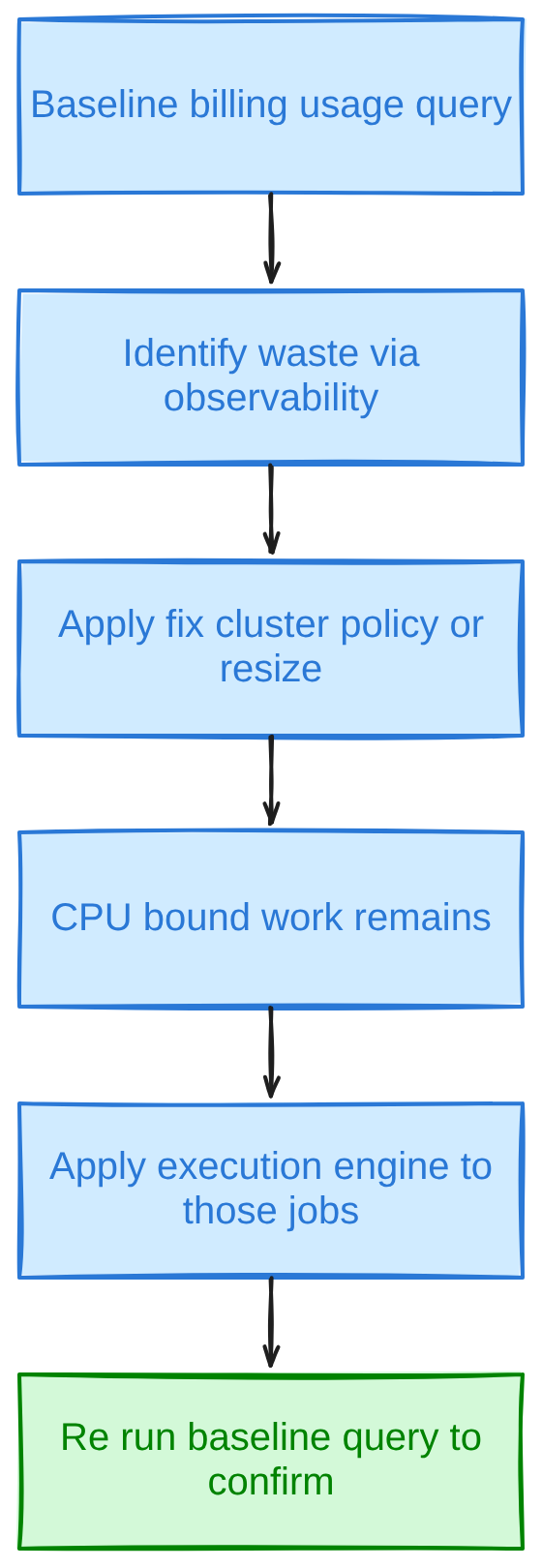
The first step is a baseline query against system.billing.usage, attributing the trailing 30 days of DBU spend by SKU and team tag before changing anything:
SELECT sku_name, usage_unit,
  SUM(usage_quantity) AS total_dbus,
  custom_tags['team'] AS team
FROM system.billing.usage
WHERE usage_date >= date_sub(current_date(), 30)
GROUP BY sku_name, usage_unit, team
ORDER BY total_dbus DESC;
Re-running the identical query after applying a fix, whether that is a cluster policy, a right-sized instance type, or an execution engine on one job, is the second step, with one caveat: because Databricks appends corrected records rather than rewriting history, a before-and-after comparison taken too close to a billing correction can look wrong for a day or two before it settles.
Which of the two to reach for first also depends on the situation in front of a team, summarized below:
| Situation | Approach that fits |
|---|---|
| No one can say which team or job drove last month’s DBU spike | Observability: start with tagging and a system.billing.usage query |
| Clusters average under 20% CPU most of the day | Observability finding plus a cluster policy fix, not a new engine |
| CPU-bound joins and aggregations dominate runtime on an already right-sized cluster | Execution engine, applied to those specific jobs |
| Pipeline failures recur several times a month and burn hours to diagnose | Observability tool with job and run-level telemetry |
| Ingestion or ELT jobs sit idle waiting on I/O for much of the run | A scheduling-aware feature of the execution layer, not a raw engine swap |
| Multiple teams share a workspace with no per-team attribution | Observability: tags and Budgets before anything else |
| A small set of jobs represents most compute-hours and the rest of the estate does not need to change | Execution engine, adopted job by job |
Pros and Cons of Observability Tools and Execution Engines
Observability tooling’s advantages and drawbacks both follow from the same trait: it watches without touching.
Observability Tools: Pros and Cons
- Surfaces exactly which job, cluster or team is spending, using data Databricks already collects.
- Catches behavioral waste, idle clusters, retries, forgotten warehouses, that no engine swap would touch.
- Low lock-in: swapping tools does not change how jobs run.
- Produces a recommendation, not a result; someone still has to act on every finding.
- Ongoing cost and attention: alerts need triage and tags need discipline to stay accurate.
- A dedicated product’s own fee often scales with the DBU spend it is watching.
Execution Engines: Pros and Cons
Execution engines approach Databricks optimization from the opposite direction: they act without watching.
- Cuts compute-hours directly on the jobs it runs, with no dashboard step in between.
- Gains are measurable in wall-clock time on day one, not dependent on someone else acting.
- Several native engines claim no application code changes, lowering the validation bar for a single job.
- Gains concentrate on CPU-bound stages; a query dominated by shuffle or short-running SQL sees less from vectorization alone.
- A higher DBU rate can offset part of the saving if the speedup is not large enough.
- Says nothing about which of the estate’s other jobs needs attention next; that is still an observability question.
How Yeedu Combines a Faster Execution Engine with Cost Visibility
Yeedu is an execution engine built on a re-engineered Apache Spark runtime, and it reports being faster across job types, not only on the CPU-bound share of a workload mix. Turbo runs multi-threaded and keeps every available core working in parallel, regardless of whether a given stage is CPU-bound, I/O-bound or a mix of both. For ingestion, ELT and streaming jobs specifically, Smart Scheduling detects idle CPU windows during read and write waits and packs tasks into them; Yeedu reports 2-4x higher cluster efficiency on that workload class. Spark-submit multiplexing runs many spark-submit jobs inside one shared, long-lived Spark session, so a dataset cached by one job serves later jobs from memory instead of a fresh read from object storage, and the Turbo Parquet disk cache keeps a local disk copy of Parquet data so repeat reads come from local disk rather than object storage.
The Turbo engine itself is a C++, vectorized, SIMD-accelerated execution layer that preserves Spark compatibility while rewriting query plans and caching at the CPU’s L2 and L3 level instead of the JVM heap. On CPU-bound work (joins, aggregations, multi-stage transforms and ML feature preparation, roughly 30 to 40% of a typical mix), Yeedu reports 4-10x faster execution and 60-80% lower compute cost, with no code changes to the Spark job itself. Yeedu’s TPC-DS benchmark completed all 99 of 99 queries at $0.52 for 1TB and $2.33 for 3TB of compute cost for that run; TPC-DS is a synthetic decision-support benchmark, and those figures are the compute cost of that specific benchmark run on the configuration Yeedu documents on its benchmark page, not a general price per terabyte for an arbitrary workload.
Yeedu also gives real-time per-job cost visibility as a built-in platform feature, and Yeedu Assistant, also branded Assistant X, adds Spark-specific diagnosis on top of it: for a failed or slow job, it can pull the job’s Spark logs, read the Spark History Server event data for that run, retrieve the cluster monitoring details, and apply root-cause analysis to explain why the job failed and recommend a fix. That is a capability of the platform running the job, not a replacement for a dedicated observability layer watching freshness, lineage or spend across an estate Yeedu is not running; the two sit alongside each other rather than overlapping.
Commercially, Yeedu runs on a fixed-price, unlimited-usage license rather than a per-core, per-hour or per-job meter, inside the customer’s own cloud account on AWS, Azure, GCP, Oracle Cloud or on-premises servers. It reads Unity Catalog, Hive Metastore and AWS Glue directly through a federated BYOCatalog layer rather than migrating metadata, so governance stays where it already is, and existing observability stacks built on Grafana, CloudWatch or Splunk keep working against the jobs that move.
Adoption follows the job, not the platform: individual Spark jobs run on Yeedu alongside Databricks, Cloudera or Amazon EMR, whichever an estate is already running, while the rest of the estate, including every job that has not moved, continues to run unchanged.
Conclusion
Databricks cost rarely has one cause, so it rarely has one fix. Observability finds where spend and failures concentrate; an execution engine cuts the compute-hours once that waste is gone.
- Data observability (freshness, schema, lineage) and cost/performance observability (DBU attribution, job and cluster telemetry) are different jobs, often bought as different products.
- Databricks ships a working slice of cost observability natively: system tables, Query Profile, Budgets, tags and cluster policies.
- Observability tools find configuration and behavioral waste: idle or oversized clusters, untagged spend, failed-and-retried jobs, warehouses left running.
- Execution engines cut compute-hours on CPU-bound work already running on a right-sized cluster; the gain has to beat any higher DBU rate the engine itself carries.
- Neither layer replaces the other: a faster engine does not explain last month’s bill, and a dashboard does not make a query run faster by itself.
- Measure before and after with the same system-table query, and account for Databricks’ retroactive billing corrections when timing that comparison.
FAQs
What are data observability tools for Databricks?
These are products, or native platform features, that monitor a Databricks estate without changing how any job runs. The category splits in two: data observability watches table freshness, volume, schema and lineage, while cost and performance observability watches job and cluster telemetry, DBU attribution and query diagnostics. Both produce a finding that a person still has to act on.
Can an observability tool reduce Databricks costs on its own?
Not directly. An observability tool surfaces where spend concentrates, such as an idle cluster or an untagged job, but the saving only materializes once someone resizes the cluster, fixes the tag or retires the warehouse. Pairing the tool with a cluster policy or a scheduled remediation closes that gap, but the tool itself only ever produces a recommendation.
What is an execution engine in Databricks?
An execution engine is the layer that turns an optimized Spark query plan into actual CPU work. Databricks’ own classic compute offers a choice between standard JVM Spark and Photon, a vectorized C++ engine enabled by default; open-source alternatives such as Apache Gluten and DataFusion Comet plug into Spark the same way on self-managed clusters. Swapping engines changes runtime and compute-hours, not which job was most expensive to begin with.
Do I need both an observability tool and a faster execution engine?
Most estates benefit from both, used in sequence rather than as a choice between them. Observability finds where hours and failures concentrate: untagged spend, idle clusters, retried jobs. An execution engine then cuts the compute-hours that remain once that waste is gone, concentrated on the CPU-bound jobs already running on a right-sized cluster. Skipping the first step risks accelerating a job that should have been fixed instead.
Are Databricks system tables enough for cost monitoring?
For a lot of the basics, yes. system.billing.usage, system.compute.node_timeline and system.lakeflow.job_run_timeline cover DBU attribution, cluster utilization and job run history natively, and Budgets and cluster policies add alerting and prevention on top. What they leave out is synthesis: cross-job root-cause correlation, anomaly alerting tuned to a team’s own baseline, and SQL-warehouse or serverless-compute coverage, which node_timeline does not include.
How do I measure whether a Databricks optimization actually saved money?
Run the same system.billing.usage query before and after the change, filtered to the same SKU and tag, over comparable time windows. Wait beyond the roughly 12-hour landing delay for new usage records, and account for the fact that Databricks appends corrected records rather than rewriting history after a billing correction, so a comparison taken right at a billing-period boundary can look off for a day or two before it settles.
What is the difference between data observability and cost observability?
Data observability watches whether tables are correct: freshness, volume, schema and lineage. Cost observability watches whether the compute producing those tables is efficient: DBU attribution, cluster utilization and query-level diagnostics. A table can pass every data-quality check while the cluster that built it ran for three times longer than necessary, which is why the two usually need separate monitoring even inside the same platform.