

Finding the three jobs responsible for half a Databricks bill is a SQL problem before it is a cost-governance problem, and Databricks system tables are where that SQL gets written. The expensive jobs surface by joining system.billing.usage to the job tables in the system.lakeflow schema and ranking the result by DBU consumption and estimated list cost, and every query below runs as written once those schemas are turned on.
One number worth carrying into that work: Databricks system tables document usage rows as “typically available within 12 hours”, and only for the ORIGINAL record type, so a query run against today’s data will always look lighter than it actually is. Once a ranking exists, three things can happen to the job sitting at the top of it: it gets tuned, it gets moved onto a different cluster shape, or it gets pointed at a different execution layer entirely, such as Yeedu's TPC-DS run completing 99 of 99 queries at $0.52 per terabyte and $2.33 for three terabytes in compute cost for that synthetic benchmark. That figure describes one benchmark, not a specific bill.
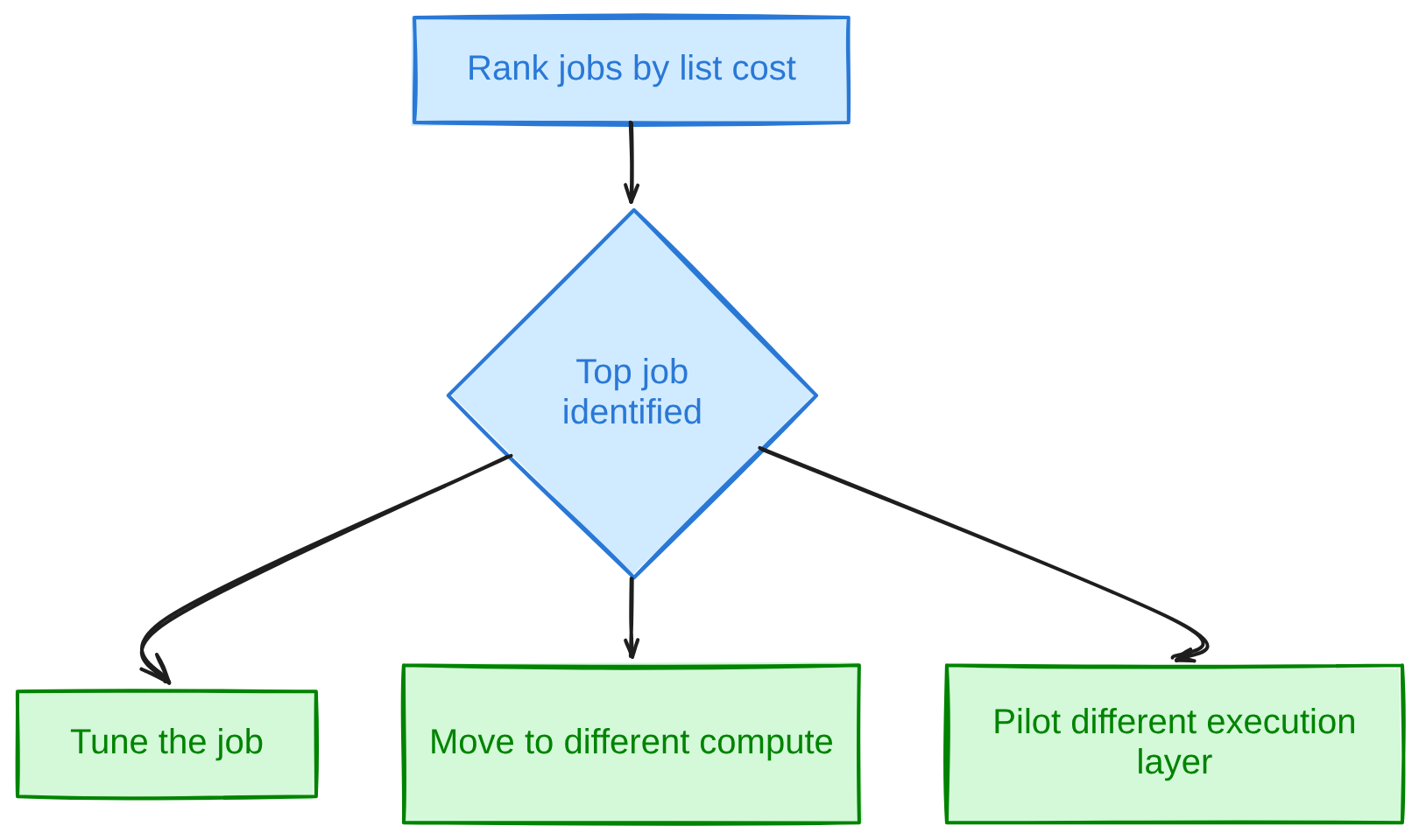
Outcomes after ranking the most expensive job
None of this requires a new tool. It requires knowing which tables exist, which columns they actually carry, and which joins quietly inflate or deflate the number that comes out the other end.
Databricks System Tables: Prerequisites and Schema Status
Databricks system tables are read-only tables that live in a reserved system catalog, governed by Unity Catalog, and populated automatically with operational data about an account rather than data a team wrote there itself. Two prerequisites gate access to all of them: the workspace has to be enabled for Unity Catalog, and the metastore behind it needs to be on Unity Catalog Privilege Model Version 1.0, a requirement stated directly on Databricks’ own reference for these tables.
Account admins and metastore admins get access by default. Everyone else needs USE CATALOG on system, USE SCHEMA on the relevant schema, and SELECT granted explicitly, schema by schema. Data is stored in a Databricks-hosted account in the same cloud region as the metastore, and it covers every Unity Catalog-enabled workspace in that region, not only the one a query happens to run from.
Schemas are not on by default, and there is no plain SHOW SCHEMAS for this; enablement is done through the account console, the REST API, or the CLI, one schema at a time, by an account or metastore admin. GA, Public Preview, and Beta status is flagged per table rather than per schema, so a schema this guide relies on for cost, such as compute or lakeflow, can still contain individual Preview or Beta tables alongside GA ones. Check the status of the specific table in the live reference before building a dashboard on it, since a Preview table can change shape without the same notice a GA one gets.
The Billing Schema: system.billing.usage and system.billing.list_prices
system.billing.usage is the row-per-usage-record table most cost queries join against, and every other query in this guide builds on it. Each row carries usage_start_time, usage_end_time, and usage_date in UTC, a decimal usage_quantity, a usage_unit (typically DBU), a sku_name, a billing_origin_product, and a record_type of ORIGINAL, RETRACTION, or RESTATEMENT.
In Databricks system tables, usage records carry their identifiers inside a struct called usage_metadata: job_id and job_run_id for job workloads, cluster_id for non-serverless compute only, warehouse_id for SQL warehouses, and dlt_pipeline_id for pipelines. Serverless workloads never populate cluster_id, and a cluster running mixed driver and worker instance types produces one usage row per node type rather than one row per cluster, which matters the moment someone tries to count clusters instead of summing rows.
system.billing.list_prices turns a DBU count into a dollar figure, with a catch: it adds a new row every time a SKU’s price changes, defined by a price_start_time and price_end_time window, so there is no single “current price” row to join against. Its pricing struct carries default, promotional, and effective_list keys: default is documented for simple long-term estimates, while effective_list is the field Databricks’ own reference uses for calculating cost, resolving promotional pricing against list pricing. Joining the two tables means matching sku_name and cloud, then landing the usage row’s usage_start_time inside the price’s validity window:
-- Price-the-usage join: list cost within the SKU's validity window
SELECT
  u.*,
  u.usage_quantity * lp.pricing.effective_list.default AS list_cost
FROM system.billing.usage u
JOIN system.billing.list_prices lp
  ON u.sku_name = lp.sku_name
 AND u.cloud    = lp.cloud
 AND u.usage_start_time >= lp.price_start_time
 AND (u.usage_start_time < lp.price_end_time OR lp.price_end_time IS NULL)
WHERE u.usage_date >= current_date() - INTERVAL 30 DAYS;
Read the output as list_cost, not as a bill. effective_list is the published rate, not a negotiated or committed one, and an Altimate.ai audit of these tables put it plainly: contracted rates, commitments, credits, taxes, corrections and cloud infrastructure costs all sit between list price and the invoice. Treat everything this guide produces as a ranking and an estimate, built for finding the heaviest jobs, not for reconciling against finance.
System Tables Databricks Queries for Your Most Expensive Jobs
The eight queries below run against Databricks system tables and cover ranking jobs, tracking their trend, catching scheduled work on the wrong compute, finding idle clusters, attributing spend, catching failed runs that still cost money, and ranking SQL warehouse queries and SKUs. Each one is written against the tables and columns described above and is complete enough to paste into a SQL editor as is.
1. Most expensive jobs by DBU and list cost
WITH latest_job AS (
  SELECT *, ROW_NUMBER() OVER (PARTITION BY workspace_id, job_id ORDER BY change_time DESC) AS rn
  FROM system.lakeflow.jobs
),
job_cost AS (
  SELECT
    u.workspace_id AS workspace_id,
    u.usage_metadata.job_id AS job_id,
    SUM(u.usage_quantity) AS dbus,
    SUM(u.usage_quantity * lp.pricing.effective_list.default) AS list_cost
  FROM system.billing.usage u
  JOIN system.billing.list_prices lp
    ON u.sku_name = lp.sku_name AND u.cloud = lp.cloud
   AND u.usage_start_time >= lp.price_start_time
   AND (u.usage_start_time < lp.price_end_time OR lp.price_end_time IS NULL)
  WHERE u.usage_metadata.job_id IS NOT NULL
    AND u.usage_date >= current_date() - INTERVAL 30 DAYS
  GROUP BY 1, 2
)
SELECT j.name AS job_name, jc.workspace_id, jc.job_id, j.creator_user_name AS created_by, jc.dbus, jc.list_cost
FROM job_cost jc
LEFT JOIN latest_job j ON jc.workspace_id = j.workspace_id AND jc.job_id = j.job_id AND j.rn = 1
ORDER BY jc.list_cost DESC
LIMIT 20;
Read job_name and created_by as context, dbus as the raw signal, and list_cost as the ranking column. The LEFT JOIN matters: if a job was deleted, its usage rows still exist but job_id no longer resolves in system.lakeflow.jobs, and an inner join would drop that spend out of the ranking silently.
2. Cost per run and the weekly trend
WITH job_spend AS (
  SELECT
    u.workspace_id AS workspace_id,
    u.usage_metadata.job_id AS job_id,
    u.usage_date,
    u.usage_quantity * lp.pricing.effective_list.default AS list_cost
  FROM system.billing.usage u
  JOIN system.billing.list_prices lp
    ON u.sku_name = lp.sku_name AND u.cloud = lp.cloud
   AND u.usage_start_time >= lp.price_start_time
   AND (u.usage_start_time < lp.price_end_time OR lp.price_end_time IS NULL)
  WHERE u.usage_metadata.job_id IS NOT NULL
)
SELECT
  workspace_id,
  job_id,
  SUM(CASE WHEN usage_date >= current_date() - INTERVAL 7 DAYS THEN list_cost END) AS last_7_day_spend,
  SUM(CASE WHEN usage_date >= current_date() - INTERVAL 14 DAYS
            AND usage_date <  current_date() - INTERVAL 7 DAYS THEN list_cost END) AS prior_7_day_spend
FROM job_spend
GROUP BY workspace_id, job_id
ORDER BY last_7_day_spend DESC
LIMIT 100;
Swap job_id for job_run_id in the same query and the grain shifts from cost per job to cost per run, which is how a job that is expensive once gets separated from a job that is getting more expensive every week. Compare last_7_day_spend against prior_7_day_spend for the growth signal, capped here at the top 100 rows so the list stays usable.
3. Scheduled work running on the wrong compute
SELECT
  u.usage_metadata.job_id AS job_id,
  u.sku_name,
  SUM(u.usage_quantity) AS dbus
FROM system.billing.usage u
WHERE u.usage_metadata.job_id IS NOT NULL
  AND u.sku_name LIKE '%ALL_PURPOSE%'
GROUP BY 1, 2
ORDER BY dbus DESC;
A populated job_id next to an All-Purpose Compute SKU name means a scheduled job is attached to an interactive cluster instead of a job cluster. It tends to be the single most common finding in a first pass over these tables, because an all-purpose cluster someone spun up for a notebook quietly became the production schedule.
4. Idle clusters
SELECT
  cluster_id,
  AVG(cpu_user_percent + cpu_system_percent) AS avg_cpu_busy_pct,
  AVG(mem_used_percent) AS avg_mem_used_pct,
  AVG(cpu_wait_percent) AS avg_cpu_wait_pct
FROM system.compute.node_timeline
GROUP BY cluster_id
HAVING AVG(cpu_user_percent + cpu_system_percent) < 10
ORDER BY avg_cpu_busy_pct;
node_timeline is minute-granularity, so add a trailing-window filter on its timestamp column before running this against the full retention period. Read avg_cpu_wait_pct carefully: a cluster with low cpu_user_percent and low cpu_system_percent but high cpu_wait_percent is waiting on I/O, not sitting idle. That is a different finding from a cluster where all three numbers are low, which is the one actually worth shrinking or terminating.
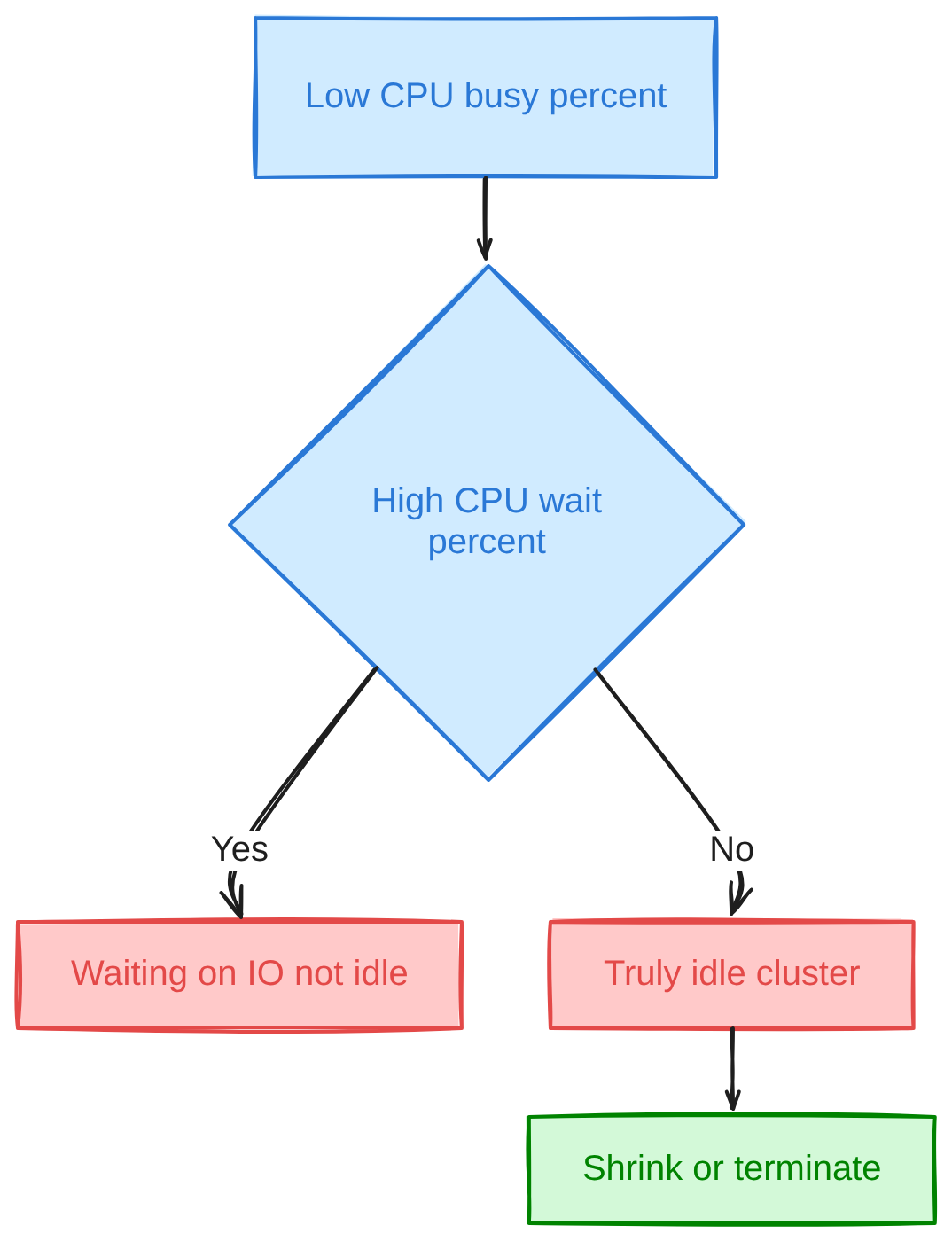
Distinguishing an idle cluster from one waiting on IO
5. Cost by owner, team, and tag
SELECT u.record_id, c.cluster_id,
  max_by(c.owned_by, c.change_time) AS owned_by,
  any_value(u.usage_start_time) AS usage_start_time,
  any_value(u.usage_quantity) AS usage_quantity
FROM system.billing.usage u
JOIN system.compute.clusters c
  ON u.usage_metadata.cluster_id = c.cluster_id
 AND c.change_time <= u.usage_start_time
WHERE u.usage_metadata.cluster_id IS NOT NULL
GROUP BY 1, 2;
That resolves ownership as of the time the compute actually ran, which matters because clusters.owned_by can change over a cluster’s life. For tag-based attribution, the equivalent is grouping by custom_tags[:key]; for the unattributed remainder, usually the more interesting finding than any single team’s number, run the same query filtered to custom_tags[‘team’] IS NULL.
6. Failed and retried runs that still cost money
SELECT
  rt.job_id,
  rt.result_state,
  COUNT(*) AS runs,
  SUM(u.usage_quantity) AS dbus_spent
FROM system.lakeflow.job_run_timeline rt
JOIN system.billing.usage u
  ON u.usage_metadata.job_id = rt.job_id
 AND u.usage_metadata.job_run_id = rt.run_id
WHERE rt.result_state IN ('FAILED', 'TIMED_OUT', 'ERROR')
GROUP BY 1, 2
ORDER BY dbus_spent DESC;
result_state also includes SUCCEEDED, SKIPPED, CANCELLED, BLOCKED, and NULL for an intermediate row of a still-running job; filtering to the failure states isolates compute spent on work that never produced an output. For multi-task jobs, the equivalent at task grain lives in system.lakeflow.job_task_run_timeline, since the duration columns on job_run_timeline are only populated for legacy single-task jobs.
7. Most expensive SQL warehouse queries
SELECT
  statement_id,
  compute.warehouse_id AS warehouse_id,
  execution_duration_ms,
  read_bytes,
  spilled_local_bytes,
  shuffle_read_bytes,
  statement_text
FROM system.query.history
WHERE compute.type = 'WAREHOUSE'
ORDER BY execution_duration_ms DESC
LIMIT 50;
statement_text returns <REDACTED> unless the caller is an admin or in the configured PII-access group, and compute.warehouse_id is only populated when compute.type is WAREHOUSE. spilled_local_bytes and shuffle_read_bytes separate a query that is slow because it is big from one that is slow because it is spilling to disk. Join the same compute.warehouse_id back to usage_metadata.warehouse_id in system.billing.usage to put a DBU figure next to the duration.
8. Spend by SKU
SELECT
  sku_name,
  SUM(usage_quantity) AS dbus,
  SUM(usage_quantity * lp.pricing.effective_list.default) AS list_cost
FROM system.billing.usage u
JOIN system.billing.list_prices lp
  ON u.sku_name = lp.sku_name AND u.cloud = lp.cloud
 AND u.usage_start_time >= lp.price_start_time
 AND (u.usage_start_time < lp.price_end_time OR lp.price_end_time IS NULL)
GROUP BY sku_name
ORDER BY list_cost DESC;
This is the line-item view: Photon SKUs, serverless SKUs, jobs compute, and all-purpose compute sitting side by side by estimated cost. Databricks’ own SKU-group documentation, self-dated February 2024, names SKUs like “AWS Premium Jobs Compute (Photon)” and “AWS Enterprise All-Purpose Compute (Photon)” but defers the actual dollar-per-DBU rate to its pricing calculator, so treat the dollar figure here as current to the day the query ran rather than as a quote.
What System Tables Cannot Tell You
System tables are the measurement layer for Databricks observability: they record what ran and what it cost, not why a particular query took the time it did. A job showing high list_cost and high execution_duration_ms tells you where to look, not what to fix.
For that, the plan-level work still happens in the query profile and the Spark UI: stage-by-stage task skew, spill, shuffle partition counts, and the physical plan Catalyst actually chose. system.query.history gives aggregate totals for spill and shuffle, but reading a skewed stage or a broadcast join gone wrong still means opening the plan itself. Treat the two as a pair: system tables tell you where to spend the time, the query profile tells you what to change.
Things That Quietly Break These Queries
A handful of details turn a correct-looking query against these tables into a wrong number, and all of them show up eventually.
Usage records arrive late, so any query touching the last day or two of usage_date will undercount, and only ORIGINAL rows are counted at all until a RETRACTION or RESTATEMENT lands. Every timestamp across these tables is UTC, which matters the moment a dashboard renders in a local timezone without converting first. Serverless usage rows never carry cluster_id, so a cluster-keyed attribution query silently drops that spend, and serverless DLT usage is tracked through dlt_pipeline_id instead, which is its own separate gap if nobody joins on it.
A deleted job leaves its usage rows in place with a job_id that no longer resolves in system.lakeflow.jobs, which is the reason every job-cost query above uses a LEFT JOIN rather than an inner one. Retention is documented and finite, not permanent: the lakeflow job tables keep 365 days, with the most recent record per entity retained past that window, while audit log rows for a workspace disappear entirely when that workspace is deleted. Querying system tables is itself billed compute, so a dashboard that re-scans 365 days of node_timeline on every refresh adds its own line item to the bill it is trying to explain.
The same job_id can appear in more than one workspace, so an account-wide ranking needs workspace_id in the grouping key, not job_id alone. The same Altimate.ai audit flags a related fan-out: joining a billing row to job_task_run_timeline on job_id alone, with no shared time bucket, multiplies every usage row across every task run and can double or triple the total. Aggregating both sides to the same grain before joining is the fix, and closing one period and confirming the total didn’t move is the validation step worth keeping. Finally, the exact table and column names here are AWS’s; Azure and GCP documentation pages exist separately and occasionally diverge, so check the page for the cloud actually in use.
From Query to Action
Each finding above maps to a specific, mostly mechanical fix, and none of it requires guessing. This section is about measurement turning into a decision, not a Databricks cost optimization playbook in its own right: the queries establish what is expensive, and the action that follows is a separate, smaller judgment call.
| Finding | Typical workload shape | Action |
|---|---|---|
| Scheduled job on an All-Purpose Compute SKU | Any scheduled batch or streaming job | Attach it to a job cluster instead of an interactive one |
| Cluster idle between runs, low CPU and memory | Ad hoc or development clusters | Enforce auto-termination through a cluster policy; practitioner defaults cited are around 30 minutes for all-purpose clusters and 10 minutes for SQL warehouses |
| Job scheduled far more often than its freshness requires | Batch ETL | Reduce the schedule; moving from daily to hourly is roughly a 5x cost increase, and to near-real-time roughly 60x, per one practitioner cost audit |
| Unattributed spend above a meaningful share of the bill | Any account without enforced tagging | Require custom_tags on cluster and job creation before optimizing anything else |
| A CPU-bound job already right-sized and still the top line item | Joins, aggregations, multi-stage transforms | Pilot it on a different execution layer, such as Yeedu or Amazon EMR, rather than another configuration change |
That last row is a different category of fix from the rest. Everything above it is configuration: a policy, a schedule, a tag. Once a job is already tuned and still expensive, the remaining lever is the execution engine itself, not the dashboard.
Operationalizing the Queries
A query that runs once during an audit and never again decays into institutional memory within a quarter. The practical version of system tables Databricks deployments actually benefit from is a saved dashboard, not a one-off notebook: schedule the top-20 job query and the SKU breakdown to refresh daily, and keep the output somewhere the team that owns the bill actually looks.
Pair the dashboard with a threshold alert on the weekly growth query from section one, rather than relying on someone to remember to open it. A job whose last_7_day_spend crosses some fixed multiple of prior_7_day_spend is a reasonable trigger. Whoever owns FinOps or platform engineering should review the ranking on a fixed cadence, monthly at minimum, since cost shape changes faster than most teams revisit it.